Background
We all have dreams. Building a home; growing a business; traveling; sending children to college; retiring comfortably. To realize these dreams, people and businesses often turn to the financial markets to help protect and grow their assets. Unfortunately, the value of stocks, bonds, and other securities fluctuates with market conditions. There are no guarantees.
Consequently, businesses, individuals, and even governments partner with experts such as Principal® to help find the best investments to achieve their goals. As the world grows smaller through commerce and technology, it’s important to have the most objective and informed perspectives to determine when and where to invest.
Analysts rely on a mix of quantitative and qualitative methodology to help investors weather the market’s ups and downs. It’s not enough to be investment experts. Having the right data at the right time plays a critical role in successfully anticipating economic and environmental changes that may impact investment performance. Personalized solutions can be designed to help people live their best life today, and tomorrow.
Using the provided data sets of financial predictors and semi-annual returns, participants are challenged to develop a model that will help identify the best-performing stocks over time.
Problem Statement
Research Question: Which stocks will experience the highest and lowest returns over the next six months?
Out of the thousands of stocks in the market, small groups will experience exceptionally high or low returns. Considering stock returns as a distribution, a portfolio manager must buy the stocks on the right tail of the distribution and avoid the stocks on the left tail. The performance of an entire equity portfolio is often driven by these key investment decisions. The goal of the inaugural Principal Challenge in Analytics Innovation is to explore methodology that will increase the probability that portfolio managers identify these stocks with extreme positive or negative returns.
Each team must create a model that ranks a set of stocks based on the expected return over a forward 6-month window. This model can be a risk factor-based strategy (multi-factor model), predictive model, or any other data-based heuristic. There are many ways to approach this task and creative, non-traditional solutions are strongly encouraged. The final model will be tested on each 6-month period from 2002 to 2017.
Datasets
Teams are provided with predictors and semi-annual returns for a group of stocks from 1996 to 2017. The data is separated into two sets: stock-level attributes and market-level and macroeconomic conditions. This span of 21 years is represented as 42 non-overlapping 6-month periods. In each of the 42 time periods, roughly 900 stocks with the largest market capitalization (i.e., total market value in USD) were selected. Therefore, the selected set of stocks at each time period changes as companies increase or decrease in value. All stock identifiers have been removed and all numeric variables have been anonymized and normalized.
Training and test datasets were created by selecting a random sample of stocks at each time period. 600 stocks were sampled into the training set and the remaining 40% created the test set. Finally, all data from 2017 was allocated to the test set. These two 6-month periods will provide a final out-of-sample test of the model’s performance.
Throughout the competition, teams will be given the opportunity to evaluate their models on the test dataset. Teams can sign in and upload their predictions up to 5 times per week. The model’s performance will be calculated and reported to the team using 40% of the test data. The remaining 60% of the test data will be held for final evaluation after the competition ends. This will provide an estimate for out-of-sample performance during the competition. Teams should rely on internal model validation procedures and be careful not to optimize results to this one small section of the test dataset.
Evaluation
Consistent performance over time and varying market conditions is crucial for any financial model. Each team must test their model using an expanding window procedure. For a given time period, T, an expanding window test allows the model to incorporate all available information up to time T, to generate predictions for time T+1. For example, when predicting the stock rankings in the first half of 2016, the model can include all data from 1990 to year-end 2015. Predictions for the second half of 2016 could then include all the data from the first half of 2016. It is very important that you do not leak data points into your training set that are from a time period in or after your prediction period. This will lead to optimistic results that do not generalize to out-of-sample data.
The quality of the predicted rankings at each time period will be evaluated in two ways, described below.
- Spearman correlation: This metric will describe the relationship between the actual rankings and the predicted rankings from the model. Higher values indicate better performance.
- Top decile performance: In reality, portfolio managers will be most concerned with stocks ranked in the top 10%. The predicted top 10% ranked stocks from the model will be compared to the actual top 10% and bottom 10% observed in the future 6-month period. A good model will maximize the proportion of highly ranked stocks in the top 10% and minimize the proportion in the bottom 10%. This metric is described in more detail below.
In addition to quantitative results, entries will be judged by the clarity of the solution, the technical strength of the methodology, and the uniqueness of the approach described in the team’s research paper. The template and requirements for the research paper are provided upon registration. Six finalists will be invited to present at the challenge event held at the University of Iowa in the Spring of 2018. The quality and clarity of the presentations provides the final criteria for selecting 1st through 6th place winners.
Spearman Correlation
Spearman correlation provides a simple metric to describe how well the model is ranking the stocks at each time period. Spearman correlation is calculated using the formula below.
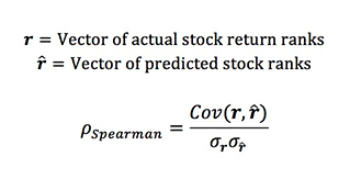
Spearman correlation has a range from -1 to 1. Models that rank stocks more accurately will produce higher Spearman correlation values.
Top Decile Performance
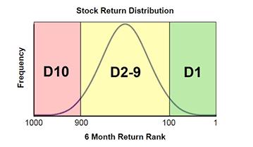
At each 6-month interval, top decile performance is calculated by the following procedure. The number of stocks changes during each time period, but for this example let’s assume there are 1000 stocks.
- Order all 1000 stocks based on the actual observed returns. (1 = highest, 1000 = lowest)
- Group the stocks into three categories. The 100 lowest returns create Decile 10, middle 800 in Decile 2-9, and the 100 highest returns in Decile 1. This is illustrated in the figure below.
- From the submitted rank predictions, subset the stocks ranked in the top 10%.
- Allocate each stock in the predicted top 10% into Decile 1 -10 based on the actual observed rank.
- Calculate the percentages of the predicted top 10% in each group. (e.g., D1: 60%, D2-9: 30%, D10: 10%)
- The final top decile score is calculated with the following function:
Based on this formulation, your objective is to create a model that correctly classifies stocks in the top 10% and avoids misclassifying bottom 10% stocks as good investments. Misclassifying a bottom 10% stocks as a top 10% is generally more costly than a correct top 10% classification is profitable. This is why the Top Decile Score applies a penalty of 1.2x the %D10, compared to the 1.0x weight applied to %D1. Stocks that fall into the middle 80% (D2-9) generally match the market returns and are therefore ignored in this score. Using the example from above where the predicted top 10% was scored as D1: 60%, D2-9: 30%, D10: 10%, the Top Decile Score would be 0.6 – 1.2*(0.1) = 0.48.
Target Group
Undergraduate students in quantitative disciplines.
A sample list includes:
- Business Analytics- Data Science
- Industrial Engineering and Operations Research
- Statistics and Actuarial Science
- Computer Science
- Mathematics
- Electrical Engineering
- Economics
- Finance & Financial Engineering
- Physics
- Computational Biology